Economics 100A
Prof. Yang

Solutions to Homework Problems                     Chapter:  1  2  3  4  5   6  7  8 9

Chapter 7

Numerical

1. Consider the model on page 178 stated below:

Y = C + I + G + X

C = 220 + 0.63 Y

I = 1,000 –2,000 R

G = 1,200

X = 525 – 0.1Y – 500R

M = (0.1583Y – 1,000 R) P

From the above equations, you can derive IS and LM curves in Equations (7.6) and (7.7)

In the textbook:

IS: R = .698 – 0.000188Y + 0.0004G (7.6)

LM: R = 0.0001583 Y – 0.001 (M/P) (7.8)

Look now in the second paragraph of page 191 under Numerical Example to see how one can derive the AD curve. As its 3^rd line says, "setting the right-hand side equations for IS and LM in Equations (7.6) and (7.8) equal and solve for Y yields:

0.698 – 0.000188 Y + 0.0004 G = 0.0001583 Y – 0.0001 (M/P)

0.0001583 Y + 0.000188 Y = 0.698 + 0.001(M/P) + 0.0004 G

0.0003463 Y = 0.698 + 0.001 (M/P) + 0.0004 G

Y = 2,015 + 2.887 (M/P) + 1.155 G à AD curve Equation (7.9)

Y = 2,015 + 2.887 (900/1.0) + 1.155 x 1,200

              = 2,015 + 2,598.3 + 1,386 =5,999.3 @ 6,000

IS: R = 0.698 – 0.000188 Y + 0.0004 G G =1,200

LM: R = 0.0001583 Y – 0.001 (M/P) M = 900; P = 1.0

IS: R = 0.698 – 0.000188Y + 0.48 LM: R = 0.0001583 Y – 0.9

Setting again the right-hand sides of the IS and LM equations and solve for Y yields the followings:

1.178 – 0.000188 Y = 0.0001583 Y – 0.9

0.0003463 Y = 2.078, Y = 6,000

R = 0.0001583 x 6,000 – 0.9 = 0.9498 – 0.9 @ 0.05 à 5%

---

Textbook Solution

a)

b) LM: R = -.0001583Y - .001M/P = .05 or 5%

IS: R = -.698 - .000188Y + .0004G = .05 or 5%

The answers agree because aggregate demand embodies the intersection of IS and LM.

c) C = 220 + .63Y = 4000.

I = 1000 - 2000R = 900.

X = 50 - .1(6000) - 500(.5) = -100.

d) 4000 + 900 + 1200 - 100 = 6000

e) D Y = 114 ® Y = 6114 ® R = 6.8% ® I = 863, X = -120.

The crowding out of investment is 37; the crowding out of net exports is 20.

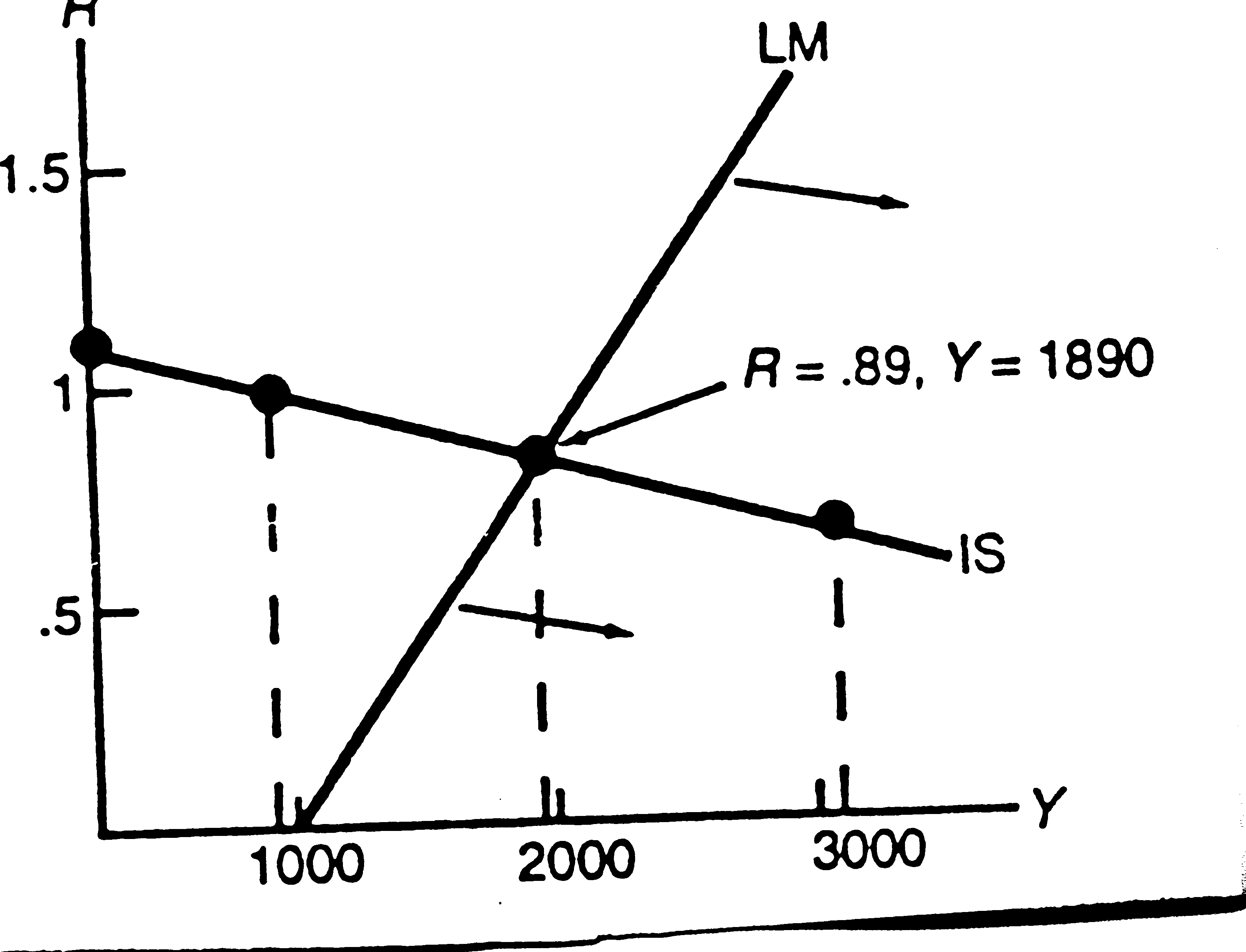
6. a) Y = C + I = 90 + .90Y + 900 - 900/R.

So the IS equation is Y = 9900 - 9000R, or R = 1.1 - (1/9000)Y. To derive the LM

equation, note that M = (.9Y - 900R)P. So the LM equation is

Y = (1/.9)M/P + 1000R = 1000 + 1000R, or R = -(1/900)M/P + .001Y = -1 + .001Y.

To find the equilibrium values of Y and R, solve the IS and LM equations for R and Y: R= .89 and Y = 1890.

If money supply increases, the LM curve shifts out and to the right.

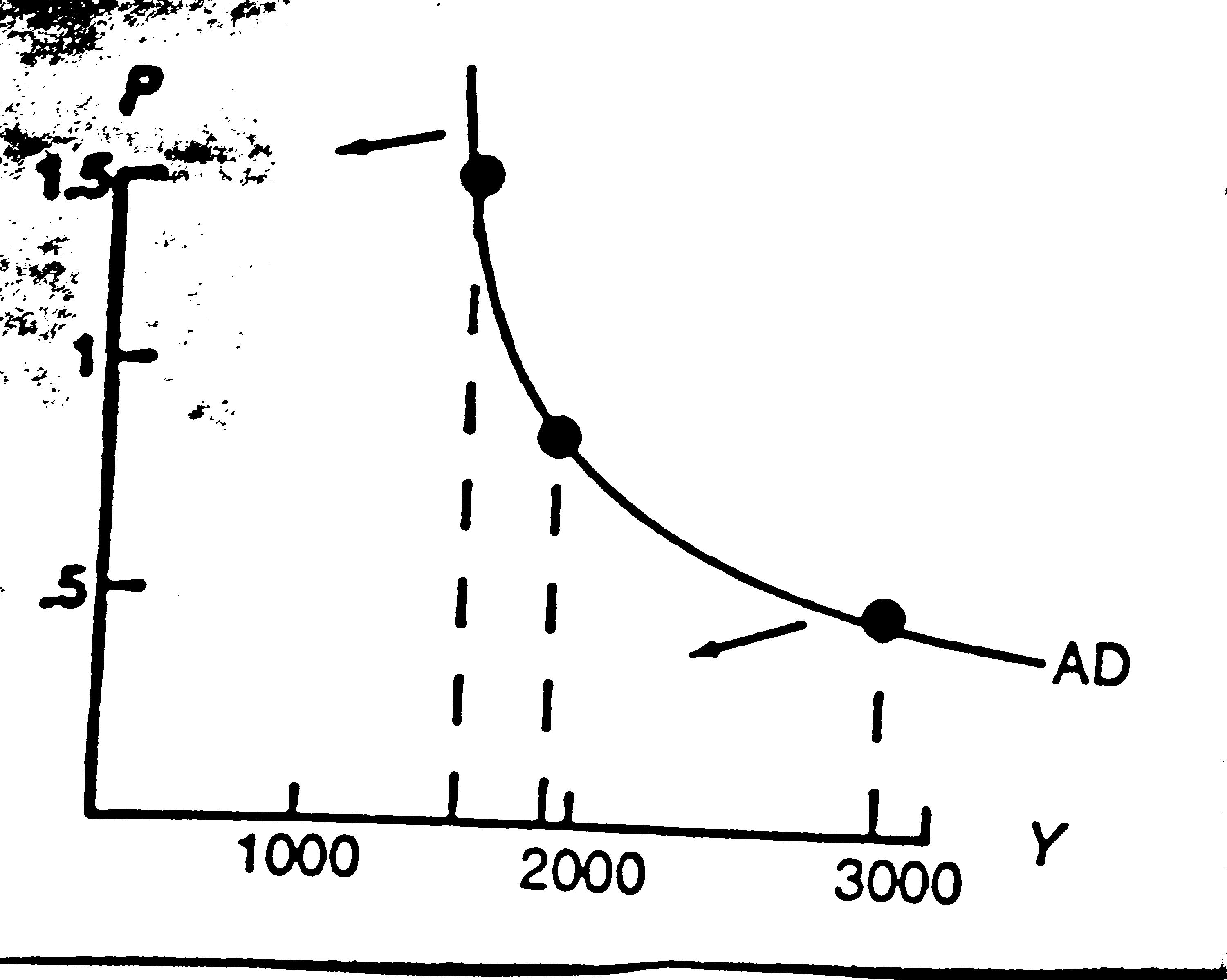
b) To get the AD curve, equate the IS and LM equations and solve for Y:

1.1 - (1/9000)Y = -(1/900)M/P + .001Y.

So the AD equation is Y = 990 - M/P = 990 - 900/P. If money supply decreases, it is clear that the AD curve will shift inward and to the left.

c) P = 900/(Y - 990).

d) Y = 1890 and R = .89