Applications of the Derivative
Derivatives
and Graphs
– Know what
it means to say that a function is increasing or decreasing on an interval.
– Know what
a critical number is and what a critical point is for a function and be able to
find then.
– Be able to
use the Increasing/Decreasing Test to find where a function f is increasing or
decreasing.
– What a
local minimum and what a local maximum is for a function f.
– Be able
to find local extrema using the first derivative test.
– Be able
to find the second derivative (or higher
derivatives) of a function f.
– Be able
to interpret the second derivative of a
function.
– Know the
concavity test.
– Know what
an inflection point is and be able to find inflection points using the second derivative.
– Be able
to find local extrema using the second derivative
test.
– Know what
an absolute maximum or absolute minimum is for a function f on an interval.
– Be able
to use the extreme value theorem to find absolute extrema.
– Be able
to set up and solve applied problems involving finding extrema.
– Make you
sure you review what the derivative f and the
second derivative f tell us about the graph of
a function f.
Analysis of Graphs
Derivatives can be used to
gather information about the graph of a function. Since the derivative
represents the rate of change of a function, to determine when a function is
increasing, we simply check where its derivative is positive. Similarly, to
find when a function is decreasing, we check where its derivative is negative.
The points where the
derivative is equal to 0 are called critical
points. At these points, the function is instantaneously constant and its
graph has horizontal tangent line. For a function representing the motion of an
object, these are the points where the object is momentarily at rest.
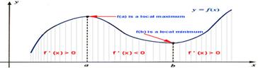
The First Derivative Test
A local
minimum (resp. local
maximum) of a function f is a point (x0, f (x0)) on
the graph of f such that f
(x0)≤f (x) (resp. f (x0)≥f (x))
for all x in some interval containing x0. Such a point is called a global
minimum (resp. global maximum) of a function f
if the appropriate inequality holds for all points in the domain. In
particular, any global
maximum (minimum) is also a local maximum (minimum).
It is intuitively clear that
the tangent line to the graph of a function at a local minimum or maximum must
be horizontal, so the derivative at the point is 0, and
the point is a critical point. Therefore, in order to find the local
minima/maxima of a function, we simply have to find all its critical points and
then check each one to see whether it is a local minimum, a local maximum, or
neither. If the function has a global minimum or maximum, it will be the least
(resp. greatest) of the local minima (resp. maxima), or the value of the
function on an endpoint of its domain (if any such points exist).
Clearly, the behavior near a local maximum is that the function increases, levels off, and begins decreasing. Therefore, a critical point is a local maximum if the derivative is positive just to the left of it, and negative just to the right. Similarly, a critical point is a local minimum if the derivative is negative just to the left and positive to the right. These criteria are collectively called the first derivative test for maxima and minima.
There may be critical points of a function that are neither local maxima nor minima, where the derivative attains the value zero without crossing from positive to negative. For instance, the function f (x) = x3 has a critical point at 0 which is of this type. The derivative f'(x) = 3x2 is zero here, but everywhere else f' is positive. This function and its derivative are sketched below.
Plot of f (x) = x3 and f'(x) = 3x2
The Second Derivative Test
Once we have found the
critical points, one way to determine if they are local minima or maxima is to
apply the first
derivative test. Another way uses the second derivative of f. Suppose x0
is a critical point of the function f (x),
that is, f'(x0) = 0. We have
the following three cases:
f''(x0) > 0 implies x0 is a local minimum f''(x0)
< 0 implies x0 is a local
maximum f''(x0)
= 0 is inconclusive
The first two of these
options derive from the observation that f''(x0)
is the rate of change of f'(x) at x0, which will be positive if the
derivative crosses zero from negative to positive, and negative is the
derivative crosses zero from positive to negative. This is called the second
derivative test for maxima and minima. The third, inconclusive case is
considered below.
The first and second
derivative tests employ essentially the same logic, examining what happens to
the derivative f'(x) near a critical
point x0. The first derivative test
says that maxima and minima correspond to f'
crossing zero from one direction or the other, which is indicated by the sign
of f' near x0.
The second derivative test is just the observation that the same information is
encoded in the slope of the tangent line to f'(x)
at x0.
Concavity and Inflection
Points
A function f
(x) is called concave
up at x0 if f''(x0)
> 0, and concave down if f''(x0)
< 0. Graphically, this represents which way the graph of f is "turning" near x0.
A function that is concave up at x0 lies above
its tangent line in a small interval around x0
(touching but not crossing at x0).
Similarly, a function that is concave down
at x0 lies below its tangent line near x0.
The remaining case is a point
x0 where f''(x0)
= 0, which is called an inflection point. At such a point the function f holds closer to its tangent line than elsewhere,
since the second derivative represents the rate at which the function turns
away from the tangent line. Put another way, a function usually has the same value
and derivative as its tangent line at the point of tangency; at an inflection
point, the second derivatives of the function and its tangent line also agree.
Of course, the second derivative of the tangent line function is always zero,
so this statement is just that f''(x0)
= 0.
Inflection points are the critical points of the first derivative f'(x). At an inflection point, a function may change from being concave up to concave down (or the other way around), or momentarily "straighten out" while having the same concavity to either side. These three cases correspond, respectively, to the inflection point x0 being a local maximum or local minimum of f'(x), or neither.
Example of Concavity and Inflection Points
Applications of the Derivative - Graphing
Temperature Fluctuation during Menstrual Cycle Maxima, Minima, and Critical Points
Graphing Polynomials Second Derivative and Concavity Points of Inflection
This section examines applications of the
derivative to finding maxima and minima. The derivative is valuable for
interpreting important aspects of graphs and biological problems. The first
problem examines a study of the body temperature of a female during the
menstrual cycle and using that to determine fertility. These ideas are
generalized to more classical Calculus applications, where the derivative is
used to help with sketching the graph of a function.
Body Temperature Fluctuation during the Menstrual Cycle
Mammals are warm-blooded and carefully
regulate their body temperature in a narrow range to maintain optimal
physiological responses. Variations in body temperature occur during exercise,
stress, infection, and other normal situations, but through neurological
control, the body self-regulates to maintain a fairly constant temperature.
Still there are slight variations including circadian rhythms where each day
the body oscillates a few tenths of a degree Celsius (minimum during times of
sleep and maximum usually occurring late in the morning). Women also experience
a normal body temperature cycle along with their menstrual cycle. Some women
monitor their basal body temperature to try to determine their peak period of
fertility to maximize (or minimize) the chance of pregnancy. The onset of
ovulation often corresponds to the sharpest rise in temperature, which gives
peak fertility. (Some claim that by the time a women notices her rise in
temperature, she is past her peak fertility, so this type of monitoring is not
universally recommended.)
Below is a graph of the basal body
temperature taken at the same time each day for a one 28-day period of one
woman. The data are fit by a cubic polynomial.
The best cubic polynomial fitting the data above is given by
T(t)
= -0.0002762 t3 + 0.01175 t2 - 0.1121 t
+ 36.41.
From the curve above we want to find the high
and low temperatures, then determine the time of peak fertility by finding the
time when the temperature is rising most rapidly.
The high and low temperatures occur where the
tangent to the curve has a slope of zero. This is where the derivative is zero.
From the rules of differentiation, we find the derivative of the temperature.
T '(t)
= -0.0008286 t2 + 0.02350 t - 0.1121.
Note that the derivative is a different function from the original function.
The roots of this quadratic equation are readily found. They are t =
6.069 and 22.29
days.
Inserting these values in the original function give
Minimum at t = 6.069 with T(6.069) = 36.1 oC Maximum at t = 22.29 with T(22.29) = 36.7 oC,
which means that there is only a 0.6 oC difference between the high and
low basal body temperature during a 28 day menstrual cycle by the approximating
function. The data varied by 0.75 oC.
The day with the maximum increase in temperature is where the derivative is at a maximum. This is the vertex of the quadratic function, T '(t). Clearly, the maximum can be found by the midpoint between the roots of the quadratic equation. However, we can also use the derivative of T '(t) or the second derivative of T(t). The second derivative is given by T "(t) = -0.0016572 t + 0.02350.
The second derivative is zero at the maximum of T '(t), which occurs at the
Point of Inflection at t = 14.18 with T(14.18) = 36.4 oC.
The maximum rate of change in body temperature is T
'(14.18) = 0.054 oC/day.
This model suggests that the peak fertility occurs on day 14, which is consistent with what is known about ovulation.
Maxima,
Minima, and Critical Points
The example above shows that finding when the derivative is zero can give
important information about the graph of a function. Another way to view this
phenomenon is to examine any graph of a smooth
function (which is a function that is continuous and differentiable). It
is clear that when you are at a
Definition: A smooth function f(x) is said to be increasing on an interval (a,b) if f
'(x) > 0 for all x in the interval (a,b).
Similarly, a smooth function f(x) is said to be decreasing on an interval (a,b) if f
'(x) < 0 for all x in the interval (a,b).
A high point of the graph is where f(x)
changes from increasing to decreasing, while a low point on a graph is where f(x)
changes from decreasing to increasing. In either case, the derivative passes
through zero.
Definition: A smooth function f(x) is said to have a local maximum at a point c, if f '(c) = 0 and f
'(x) changes from positive
to negative for values of x near c. Similarly, a smooth function f(x)
is said to have a local minimum
at a point c, if f '(c) = 0 and
f '(x)
changes from negative to positive for values of x near c.
Clearly, it is important to find where the
derivative is zero to find these highest and lowest points on a graph.
Definition: If f(x) is a smooth function with f '(xc)
= 0, then xc is
said to be a critical point of
f(x).
Finding critical points helps find the local
high and low points on a graph, but some critical points are neither maxima or
minima.
We applied these definitions to a cubic function describing body temperature over a month. Let us examine how finding critical points can help us graph other polynomials. Consider the following examples.
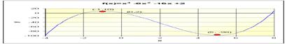
Example: Suppose that f(x) = x3 - 6x2 - 15x + 2.
Use the information to help sketch a graph of f(x).
Solution: We begin by taking the derivative, f '(x) = 3x2 - 12x - 15
= 3(x + 1)(x - 5).
The derivative is zero when xc = -1
or 5. Evaluating the function at the
critical points, we find f(-1) = 10, which gives a local maximum at (-1,10), and f(5) = -98, which gives a local minimum at (5,-98). The y-intercept
is (0,2) another easy point to add to our
graph, so we now have good information to make a reasonable sketch of the
graph, which is shown below. Note that since this is a cubic equation, the x-intercepts are very hard to find.
The Second Derivative and Concavity
Since the derivative is itself a function,
then if it is differentiable, one can take its derivative to find the second derivative often denoted f ''(x).
The sign of the second derivative tells where the first derivative is
increasing or decreasing. If the first derivative is increasing or the second
derivative is positive, then the original function is getting
"steeper." The function is said to be concave
upward. If the first derivative is decreasing or the second
derivative is negative, then the original function is said to be concave downward. Thus, the second
derivative is a measure of the concavity of a function. For our smooth
functions described above, we can see that maxima generally occur where the
function is concave downward, while minima occur where the function is concave
upward. This property is often summarized in the following test.
The Second Derivative Test. Let f (x) be a smooth function. Suppose that f '(xc)
= 0, so xc is a
critical point of f. If f ''(xc)
< 0, then xc is
a relative maximum. If f ''(xc) > 0, then xc is a relative minimum.
Example: If we
return to our example above where f(x) = x3 - 6x2
- 15x + 2, then we see that the second derivative is
f ''(x) = 6x - 12.
The critical points occurred at xc = -1
and 5. Evaluating the second
derivative at the critical point xc = -1, we find f ''(-1) = -18, which says the function is concave
downward at -1, so this is a relative maximum. Similarly, the second derivative
at the critical point xc = 5 is f ''(5) = 18, which says the function is concave
upward, so this is a relative minimum.
When the second derivative is zero, then the
function is usually changing from concave upward to concave downward or visa
versa. This is known as a point of inflection.
A point of inflection is where the derivative function has a maximum
or minimum, so the function is increasing or decreasing most rapidly.
In the application above for the variation of body temperature over one month
of a menstrual cycle, the point of inflection represented the potential time of
peak fertility by finding where the basal body temperature was increasing most
rapidly.
From a graphing perspective, the point of
inflection shows the visual change in concavity. It is not nearly as important
as extrema, but does provide one more point to aid in graphing the function.
Example: Once again
returning to our example above of f(x) = x3 - 6x2
- 15x + 2, where the second derivative is f ''(x) = 6x
- 12, we can easily find the point of inflection. We see that f ''(x) = 0
when x =
2. Thus, the point of inflection occurs at (2,
-44). This can be see on the graph above.![]()
Applications of the Derivative -
This section provides a series of examples to
supplement the lecture section and help with the homework problems. The first
examples examine graphing problems. The second example returns to the height of
a ball in the air, while the last example uses the derivative to find the
maximum and minimum population from a study.
Examples
of Graphing Problems: Below are two
more examples of graphing problems, where we can apply the derivative and
second derivative to help with the sketch of the graph.
Example 1: Use the techniques
developed in lecture to find any local or relative minima and maxima and points
of inflection for the following polynomial:
![]() .
.
Sketch
a graph of the function.
Solution: When you want to
sketch a graph, the most important part of sketching the graph is finding the
extrema (maxima and minima). These are found by finding the derivative and
setting it equal to zero. The solutions of the equation for the derivative
equal to zero give the critical values, which are substituted back into the the
original function. By adding the x
and y-intercepts (if possible) and
any asymptotes (if they exist) to the sketch, you can get a fairly good idea of
what the graph looks like. The second derivative provides nice information to
aid with the graph, but it's not nearly as essential in getting a good looking
graph.
The y-intercept should always be easy, and in this case, we readily see that (0, 0) is both an x and y-intercept. We can factor this equation and solve for the x-intercept. To find the x-intercept, set y = 0, then factor and solve the equation,
-x(x2 - 12) = 0 or ![]()
To find the extrema, we take
the first derivative of the function and set it equal to zero. Then we solve
for xc, where
y' = 0. y' = 12 - 3x2 = -3(x2 - 4) = -3(x + 2)(x - 2) = 0 xc = -2, 2
We evaluate the original function at the critical points, giving y(-2) = -16 and y(2) = 16, so the critical points of the function are (-2, -16) and (2, 16). Clearly, the first point is a minimum and the second is a maximum. However, we can check this with the second derivative test. We take the second derivative and evaluate at the critical points to see if they are minima or maxima. y'' = -6x
y''(2) = -6(2) = -12
is concave downward, which indicates a maximum
y''(-2) = -6(-2) = 12 is concave upward, which indicates a minimum
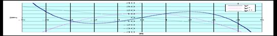
Thus the point (-2, -16) is a local minimum and the point (2, 16) is a local maximum. The points of inflection occur at the
point where the second derivative is equal to zero. In this case, the
inflection point is at x
= 0. This means that the concavity direction
changes at point (0, 0). The concavity is upward to the left of (0, 0), and downward to the right of (0, 0). The graph below shows the function and its first and
second derivatives.
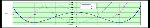
Example 2: Use the techniques developed in lecture to find the local or relative minima and maxima and points of inflection for the following polynomial: y = x4 - 8x2.
Sketch a graph of the function.
Solution: See the discussion in Example 1 about the most
important steps in sketching a graph. The steps one should always take to
create a graph are as follows:
- Find
any x or y - intercepts. (Often x - intercepts are too difficult to
find.)
- Find
any vertical or horizontal asymptotes.
- Find
extrema (local minima and maxima).
- Find
any points of inflection.
The y-intercept is easily found as
(0, 0), which is both an x and y-intercept.
We can factor the equation above and solve for the x-intercept x2(x2 - 8) = 0 or ![]()
The critical points xc can be found when the first derivative of
the function is set equal to zero.
y' = 4x3 - 16x = 4x(x2
- 4) = 4x(x - 2)(x +2) = 0
The critical points are at xc = -2, 0, 2. As before, we evaluate the function at
each of the critical points, y(-2) =
-16, y(0) = 0, and y(2) = -16,
so the critical points of the function are (-2, -16), (0, 0), and (2, -16). Clearly,
the first point is a minimum, the second is a maximum, and the third is a minimum
again.
Again we can check with the
second derivative (though usually this step can be omitted because function
evaluation gives the relative height of extrema). The nature of these critical
points can be found by evaluating the second derivative function at the
critical points of the first derivative function. If the result is negative it
indicates a maximum and if the result is positive it indicates a minimum.
y'' = 12x2 - 16 = 4(3x2
- 4) = 0 ![]() y''(-2) = 4[3(-2)2
- 4] = 32
y''(-2) = 4[3(-2)2
- 4] = 32 ![]() y''(0) = 4[3(0)2
- 4] = -16
y''(0) = 4[3(0)2
- 4] = -16 ![]() y''(2) = 4[3(2)2
- 4] = 32
y''(2) = 4[3(2)2
- 4] = 32
Thus the critical points indicate
local minima at (±2,-16) and a local maximum at (0, 0). The
inflection points occur at the zeros of the second derivative function, which
are at approximately (±1.155,
-8.889). These
characteristics are illustrated in the graph below.
Example 3: Height of the Ball
Revisited Consider a ball
that is thrown vertically with a initial upward velocity of 64 ft/sec (so v0= 64). The acceleration due to gravity is g = -32 ft/sec2. With these values, the
height of the ball satisfies
h(t) = 64 t - 16 t2.
Find how high this ball travels.
Solution: There are two good ways to solve this problem. From
our knowledge of the height function being a quadratic, we could simply find
the vertex of the parabola, knowing that it must be at the top of the flight of
the ball. Another physical property that can be used to find this maximum for flight of the ball is to
recognize that at the top of its flight the ball is temporarily stopped, then
its velocity becomes negative as the ball falls back to the ground. Thus,
finding the time when the velocity is zero gives the time of the maximum height
of the ball.
The velocity function from our differentiation rules is v(t) = 64 - 32 t.
Solving the velocity equal to zero, 64 - 32 t
= 0,
gives the critical time, t = 2 sec. The maximum height of the ball is found by substituting this critical time into the original height equation, so h(2) = 64(2) - 16(2)2 = 64 ft.
Example 4: Study of a
PopulationThe ocean water is monitored for fecal contamination by
counting certain types of bacteria in a sample of seawater. Over a week where
rain occurred early in the week, data were collected on one type of fecal
bacteria. The population of the particular bacteria (in thousand/cc), P(t),
were best fit by the cubic polynomial
P(t)
= - t3 + 9 t2 - 15 t + 40, Where
t is in days.
a. Find the rate of change in population per
day, dP/dt. What is the rate of
change in the population on the third day?
b. Use the derivative to find when the
relative minimum and maximum populations of bacteria occur over the time of the
survey. Give the populations at those times. Also determine when the bacterial
count is most rapidly increasing.
c. Sketch a graph of this polynomial fit to
the population of bacteria. When did the rain most likely occur?
Solution: a. To find the rate of change in population per day,
we take the derivative of P(t),
![]()
Evaluating this on the third day gives P '(3) = 12 (x1000/cc/day).
b. The critical points are found by setting
the derivative equal to zero. This particular quadratic factors easily, so
P '(t)
= -3 t2 + 18 t - 15 = -3(t - 1)(t - 5) =
0.
It follows that the critical values are tc = 1or 5.
Substituting the critical values into the population function, we have
Minimum at t = 1 with P(1) = 33 (x1000/cc) Maximum at t = 5 with P(5) = 65 (x1000/cc).
To find when the population of bacteria is
increasing most rapidly, we take the second derivative and set it equal to
zero. (Finding the point of inflection.) Thus, we have P "(t) = -6 t + 18 = -6(t - 3) =
0.
It follows that the population is increasing
most rapidly at t = 3 with P(3) = 49 (x1000/cc). Above we see that this maximum increase is P '(3) = 12 (x1000/cc/day).
c. Below we have the graph of this
population. Notice that the population at t = 7 with P(7) = 33 (x1000/cc), which matches the local minimum given above. From the graph, we can
guess that the rain fell on the second day of the week with storm runoff
polluting the water in the days following.