Regression
-
Equation of a Straight Line
As you will see below a regression line is a straight line that
represents the relationship between an x-variable and a
y-variable. Recall that the equation of a straight line is y = m x + b.
Quantity m gives the slope (rise/run) of the line and the y-intercept (the y
coordinate at which the straight line crosses the y axis) is given by b.
The line y = x has a slope of 1 and a y-intercept of 0 while the
line y = 3x - 2 has a slope of 3 and a y-intercept of -2. What
are the slope and y-intercept of the line whose equation is 3x -
2y + 4 = 3?
-
Regression Line
Statistical data often consists of related pairs of numbers, for example, height and weight, income and
taxes paid, age and blood pressure, or advertising expenditures
and income for a company. You can think of these pairs of numbers as the
x and y-coordinates of points in the plane. You can plot
these datapoints on a x-y coordinate system. For example,
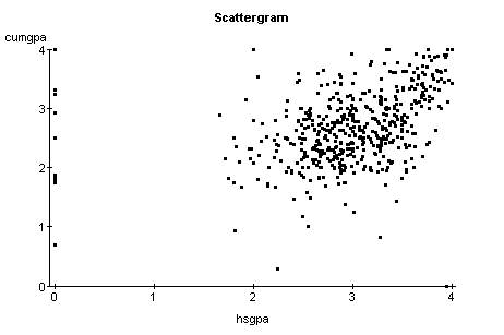
using the FOCUS dataset choosing Scatter Plot under the Graphics
menu, and then selecting High School GPA (hsgpa) as the x-variable
and Cumulative GPA (cumgpa) as the y-variable produces the
following scatterplot.

Clearly, you can't draw a single straight line that passes
through all of these points. However, you can draw a straight line that lies
approximates the relationship between hsgpa and cumgpa.
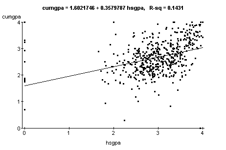
Such a line is shown in the next graph.

The equation of the regression line is shown in the
title. We will discuss R-sq later. The line shows that
generally as hsgpa increases, cumgpa increases. How is the equation of this regression line
determined? The next graph shows four given data points (in black). The points
have coordinates (1,1), (2,3), (3,3), and
(4,5). No single line will pass through all four points.
However, you can try to find lines that come close to the points.

The next four graphs show four lines (in purple)
that come close to the given points. The equations of the
lines are y=0.75x+1.5 (upper left graph), y=1.5x-1 (upper right
graph), y=1x+0.5 (lower left graph), and y=1.2x (lower right
graph). Closeness of the line to the points is measured by
the sum of squares of the vertical distances (lengths of the red
vertical segments) between the given points and points (in purple)
lying on the line vertically above or below the given points.

The sums of squares are 2.375 for the upper left
hand graph, 1.5 for the upper right hand graph, 1 for the lower
left hand graph, and 0.8 for the lower right hand graph.
Follow this link to see an Excel
spreadsheet showing sum of squares calculations.
The least squares line of best fit, called the
regression line for short, is the line that makes this sum of
squares as small as possible. For the example above, the
regression line is the line shown in the lower right hand graph,
the line y=1.2x. Calculus techniques can be used to derive
formulas for the slope and y-intercept of the regression line whose equation is denoted by
y=b1x+b0. You will only need to apply
the resulting formulas. First compute:


 For
the given points, (1,1), (2,3), (3,3), and (4,5), Sxx=(12+22+32+42)-((1+2+3+4)2/4)=30-(102/4)=30-25=5, Syy=(12+32+32+52)-((1+3+3+5)2/4)=44-(122/4)=44-36=8,
Sxy=(1*1+2*3+3*3+4*5)-((1+2+3+4)*(1+3+3+5))/4)=36-((10*12)/4)=36-30=6 Then
b1=Sxy/Sxx=6/5=1.2, and b0=(12/4)-(1.2*(10/4))=0.
So the regression line is the line shown in the lower right
hand graph shown above. Click on the orange
area below to open the FOCUS dataset within Webstat. Use
Simple Linear Regression under the Stat menu to verify the
regression calculations shown above.
Click on this link for an Excel spreadsheet
that contains the FOCUS data, a scattergram of HSGPA on the
horizontal axis, CUMGPA on the vertical axis, and the regression line,
regression equation, and the coefficient of determination (r2).
-
Coefficient
of Determination and Correlation Coefficient
Look at the Scattergram of Your Data First
You can use the equations shown above to find the regression
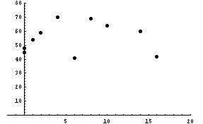
line for any set of numbers. For example, given the pairs of
numbers, (16,42), (1,54), (14,60), (4,70), (0,48), (6,41), (2,59),
(10,64), (0,45), (8,69), using the formulas shown above, the
equation of the regression line is y = 0.115653 x + 54.4945.
However, look at the scattergram of these numbers.

It appears that there isn't a linear relationship between
the x and y variables. So, before trying to compute a
regression line, which should only be used when a linear
relationship exists between the variables, make a scatterplot.
If the scatterplot makes it clear that there is not a linear
relationship between variables, don't use linear regression.
What is the Coefficient of Determination
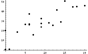
Look at the next two scattergrams.
 
In both cases, it appears that there is a linear relationship
between the x and y variables. However, if you imagine
regression lines atop the scatterplots, you can see that in the left graph
the points will lie closer to the regression line than in the
right graph. The coefficient of determination is a number
that measures the degree of closeness of points to the
regression line. This degree of closeness is called
'goodness of fit' by statisticians.
Variation in y-values is
measured by the standard deviation of the y-values. Standard
deviation is measured by

In defining the coefficient of determination, only
the inside top of this formula is used, and the x's are replaced
by y's. It is called the
total sum of squares or SST, and is given by (y with a bar over it
is the mean or average of the y-values):

It can be shown that SST can be expressed as the
sum of two terms named SSR and SSE. SSR, or the sum of
squares due to regression is given by the formula (y with
a 'hat' over it signifies a the y-value found by using the
regression equation on a x-value to find the
corresponding y-value ):

SSR measures the amount of total variation in
y-values explained by the regression line. The amount of
total variation not explained by the regression line is called the
sum of squares for error and denoted by SSE. The formula for
it is:

These three quantities are related by the formula
(which can be shown algebraically):
SST = SSR + SSE
Dividing both sides of this formula by SST results
in the equation
1 = (SSR/SST) + (SSE/SST)
In this equation SSR/SST is called the
coefficient of determination--it measures the proportion of
variation in the y values explained by the regression line.
Multiplying by 100 gives the percentage of the variation in
y-values explained by the regression. The coefficient of
determination is denoted by r2. For the data
shown in the last three graph above, the coefficient of
determination is 3046.68/3187.67 =0.96. So about 96% of
the variation in y-values is explained by the regression.
The other 4% is unexplained or error variation.
Formulas for computing SST and SSR are:


where

-
How is the Correlation Coefficient Computed
Correlation measures the degree of linear relationship between
two variables and is the square root of the coefficient of
determination. It is denoted by r and is the square root of
the coefficient of determination, r2. Since r2
can only lie between 0 and 1, r must lie between -1 and
1. Also, since values of r2near 1
indicate that the regression line lies close to the data points,
i.e. the regression line explains most of the
variation in y-values, values of r near -1 or +1 also indicate a
regression in which most of the variability in y's is explained by
the regression line. Values of r near +1 indicate a
regression line with positive slope, which implies that there is a
direct linear relationship between the x and y-variables, while
values of r near -1 indicate a regression line with negative slope
implying an indirect or inverse linear relationship between the
variables.
Another formula for computing the correlation coefficient is:

where the symbols in the formula have been defined
above.
-
Relationship between the Correlation Coefficient, the
Scattergram, and the Regression Line
This link
takes you to an interactive demonstration that shows the
relationship between the correlation coefficient and the
regression line. When the page opens click on
Interactive Scatterplot. After the simulation for the
scatterplot opens, you can place points on the display by clicking
the mouse button. After the 2nd point has been placed the
regression line will be drawn. In addition, the correlation
coefficient and other statistics will be shown. Here is a link
to another demonstration of the relationship between the
scattergram or scatterplot and the correlation coefficient.
Once the page opens click on the + symbol next to Statistical
Application--the display will change, then click on the + next to
correlation, then click on the + next to applets, and finally
click on correlation movie. When the movie plays you will
see the relationship between points in the plane and the
correlation coefficient.
Computation of Regression Lines and
Coefficients of Determination
Make the following regression calculations on the
FOCUS: database using Webstat2. You can open Webstat2 by pushing
the orange button above.
1. Make a scatterplot of the points where SAT Math is
the y-variable and SAT Verbal is the x-variable. Then find and
plot the regression line on the scatterplot of points, find the
coefficient of determination and correlation coefficient. Relate
these coefficients to the regression line plotted on the graph.
2. Do the same as in number 1 but make HS GPA the
x-variable and Cumulative GPA the y-variable.
3. Finally, answer the same questions as in 1 but use
hours as the x-variable and hsgpa as the y-variable.
|
|