PIPE FLOW: TURBULENT
BACKGROUND
Smooth & rough pipes:
Qualitative rating of pipe surface
Relative roughness:
Average roughness along pipe divided by
pipe diameter
Static heads:
Measured perpendicular to direction of flow:
(p/γ + z)
Stagnation head:
Tap pointed up-stream of flow direction:
(p/γ + z + v2/2g)
Laminar & turbulent flow
Some theory for laminar flow
Civil Engineers almost always work with
turbulent flow for pipes
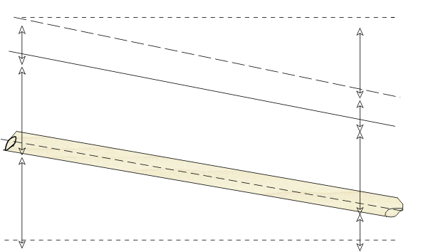
Hydraulic Grade Line In A Pipe

Energy Equation for Steady, Uniform Flow
p1/γ + z1 + v12 + hP = p2/γ + z2 + v22 + + hT + hL
Subscripts 1 & 2 are at the start and end of the flow section
hL is the head loss due to flow over a length of the pipe from points 1 & 2
hP and hT are heads associated with pumps and turbines respectively
Common Headloss Equations
Darcy-WeisbachhL = f (L/D) (v2/2g)
Hazen-Williams hL = (v/αC)1.85L/R1.17
Manning: hL = (nv/β)2 L/R4/3
R is hydraulic radius; f and n are resistance factors, and C is a conductivity factor. α and β are needed to convert for common units.
TURBULENT FLOW IN PIPES
Objectives:
To determine the friction factors associated with turbulent flow in smooth and rough pipes.
To observe and compare the velocity distributions in smooth and rough pipes.
Apparatus:
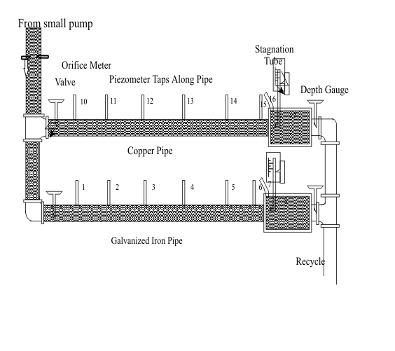
Pipe assemblies equipped with taps and a manometer board
Upstream orifice meter with differential manometer
Movable stagnation tubes and manometers fitted to the outlets of the pipes
Pipe Flow Apparatus
Pipe assemblies equipped with taps and a manometer
board
Upstream orifice meter with differential manometer
Movable stagnation tubes and manometers fitted to the
outlets of the pipes

Experimental Procedure
1. Set up the experiment.
a. Open the surge tank valve and turn on the small pump.
Release water from several valves around the lab to remove air from the piping system.
b. Measure the positions of the manometer taps along the two pipes.
c. Measure the water temperature
2. Measure head loss vs. distance and flow.
a. Establish a steady flow through one of the pipes
b. Use the back-pressure valve at the end of the pipe to control the level of the manometers
c. Record the levels for all manometers
d. Record the differential head across the orifice in the supply line
e. Convert the orifice manometer reading to flow using the rating curve provided
3. Repeat Step 2 for 6-7 flows through the subject pipe
4. Measure the velocity profile across the pipe.
5. Repeat Steps 2, 3, and 4 for the second pipe.
6. Turn off the pump and drain the pipes. Close the
surge tank valve.
Data Sheet for Turbulent Flow (1)
Calif. State Univ., Sacramento CE 135 HYDRAULICS LAB.
Dept. of Civil Engineering
TURBULENT FLOW IN PIPES
INPUT (OBSERVED) DATA
Lab. Team: Date of Experiment:
------------------------------------ CONSTANT DATA ----------------------------------------------
Water Temperature ________° F
----------------------------------- VARIABLE DATA ------------------------------------------------
PIPE TYPE: _____________________ PIPE D(in) = ________
FLOW HEAD MANOMETER HEADS (in)
Run |
H1 |
H2 |
Tube-> |
# |
# |
# |
# |
# |
# |
# |
No. |
(in) |
(in) |
X(ft)-> |
0 |
3 |
6 |
10 |
14 |
18 |
18.5 |
1 H->
Flow Gpm (H-ref->)
2 H->
Flow
3 H->
Flow
4 H->
Flow
5 H->
Flow
6 H->
Flow
7 H->
Flow
Reference Tap “H-ref”
(Optional)
Purpose: Adjust for effect of random pressure (head)
fluctuations in the pipes
Assign one of the taps, say the one at X=0, to be read at
the same time as H is read for each tap at a point
at distance 0-18.5
If both fluctuate at same time, the two points get same
change
(Not perfect, but helps)
Experimental Results (1)
Plot the piezometric head vs. pipe pressure tap position
for all flow rates and pipes.
These are used to determine the head loss - length relationship
Determine the relative roughness (ks/D)
Calculate friction factor (f) and Reynolds Number (Re)
Plot your f and Re data on a Moody diagram.
Determine the relative roughness of each pipe
Calculate the absolute roughness.
Plot a graph, at log-log scale, of f vs. Re, like the Moody
diagram
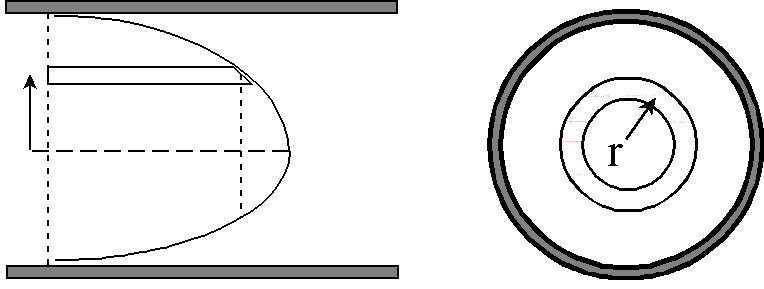
Flow From Velocity Distribution
Theoretical Equation: Q = ∫v2πrdr = 2π∫vrdr

Ideally, v is constant around the circular path at radius r. In practice, some variation can be expected.
Practical Equation: Q = ∑ vi ΔA = ∑ vi 2πri Δr
Data Sheet for Turbulent Flow (2)
Velocity Profile Data
Velocity Distribution Data: Manometer # ______
Heads for Flow: H1 ______ in H2 ______ in [Gives Q = ________ cfs]
Reading Number 1 2 3 4 5 6 7 8 9
Probe Location:
(Inch)
Stagnation Head:
(Inch)
Static Head:
(Inch)
Experimental Results (2)
Calculate values of Hazen-Williams coefficient for each
run. How good is the assumption that the coefficient is constant with Re?
Compare your measurements of absolute roughness and
Hazen-Williams coefficient with tabulated values for copper and galvanized steel pipe
Note:
Re = vD/ν = 4Q/πDν
f = 2gDhL/Lv2 = g π2D5hL/8LQ2
Hazen-Williams C = v(L/hL)0.54/0.355D0.54
Example Spreadsheet Data
CONSTANT DATA
Water Temp. 75 F Spec. Wt. 62.37 lb/ft^3
Kinem.Visc. 1.03 x 10^-5 ft^2/s
VARIABLE DATA
------------------------ Copper Pipe ------ D(in)= 2.004 ---------------------------
------- Flow Rate ------- ------------- Manometer Heads (inches) ------------
| Run | H1 | H2 | Q | Tube | 8 | 9 | 10 | 11 | 12 | 13 | 14 |
|---|---|---|---|---|---|---|---|---|---|---|---|
| No. | (in) | (in) | (gpm) | X(ft) | 0 | 3 | 6 | 10 | 14 | 18 | 18.5 |
| 1 | 1.0 | -13.0 | H(in) | 12.0 | 0.5 | 8.5 | 6.3 | 4.0 | 2.3 | 1.7 | |
| H--ref | 12.0 | 12.0 | 11.8 | 11.8 | 11.8 | 12.0 | 12.0 | ||||
| 2 | 3.3 | -20.0 | H(in) | 24.5 | 22.1 | 19.1 | 15.6 | 12.5 | 8.7 | 8.4 | |
| H-ref | 24.5 | 24.5 | 24.3 | 24.3 | 24.3 | 24.2 | 24.2 | ||||
| 3 | 3.5 | -25.5 | H(in) | 26.3 | 23.3 | 20.2 | 15.6 | 11.5 | 8.6 | 7.2 | |
| H-ref | 23.3 | 26.1 | 26.4 | 26.1 | 26.0 | 25.9 | 25.9 | ||||
| 4 | 4.0 | -28.5 | H(in) | 25.4 | 22.3 | 18.5 | 13.7 | 9.3 | 5.1 | 4.6 | |
| H-ref | 25.4 | 25.4 | 25.2 | 25.2 | 25.2 | 25.2 | 25.1 | ||||
| 5 | 2.8 | 5.2 | H(in) | 19.5 | 19.3 | 18.9 | 18.5 | 18.4 | 17.9 | 18.1 | |
| H-ref | 19.5 | 19.5 | 19.5 | 19.7 | 19.7 | 19.9 | 21.1 | ||||
| 6 | 0.0 | -9.0 | H(in) | 16.8 | 15.4 | 14.3 | 12.8 | 11.8 | 10.1 | 10.1 | |
| H-ref | 16.8 | 16.6 | 16.3 | 16.3 | 16.8 | 16.5 | 16.6 |
CE 135 HYDRAULICS LAB. FLOW IN PIPES WITH FRICTION
CALCULATIONS
COPPER (SMOOTH) PIPE
| Tap Position (ft) --> | 0 | 3 | 6 | 10 | 14 | 18 | 18.5 | |
|---|---|---|---|---|---|---|---|---|
| Run | Q (cfs) | Head Loss, Cumulative (in) | ||||||
| 1 | 0.108 | 0 | 1.5 | 3.3 | 5.5 | 7.8 | 9.6 | 10.2 |
| 2 | 0.139 | 0 | 2.3 | 5.2 | 8.6 | 11.8 | 15.5 | 15.8 |
| 3 | 0.155 | 0 | 2.8 | 6.2 | 10.4 | 11.5 | 14.5 | 17.3 |
| 4 | 0.164 | 0 | 3.1 | 6.7 | 11.5 | 15.9 | 20.1 | 20.5 |
| 5 | 0.044 | 0 | 0.2 | 0.6 | 1.2 | 1.3 | 2.0 | 3.0 |
| 6 | 0.086 | 0 | 1.2 | 2.0 | 3.5 | 5.0 | 6.4 | 6.5 |
Darcy-Weisbach and Hazen-Williams Coefficients
Run Reynolds Darcy- Hazen-
No. Number Weisbach Williams Epsilon
f C (ft)
1 0.0799 x10^6 0.0199 148 0.0375 x 10^-3
2 0.1034 0.0190 148 0.0366
3 0.1151 0.0171 155 0.0103
4 0.1218 0.0177 152 0.0130
5 0.0331 0.0239 143 0.0566
6 0.0641 0.0204 148 0.0251
Roughness values computed from Colebrook equation:
Absolute Roughness = 0.0232 x 10^-3 ft
Relative Roughness = 0.139 x 10^-3